
Application Note 4
An In-Depth Discussion of Digital Filter Options in the AMETRIX Model 100 Series Picoammeters
Glenn Fasnacht, President, AMETRIX Instruments
I. Introduction
The filters available are all digital filters; that is they filter the already acquired data. This is as opposed to analog filters that affect the analog signals before being digitized.
Filtering is made available to reduce noise in the measured data. Some filtering is offered in the Measurement Mode drop-down.
Rates of 3600, 1800, and 900 samples per second (Sa/s) are unfiltered by the AMETRIX® software, but as the sample rate is lowered, the data converter in the Model 100 Series improves the signal-to-noise ratio.
Sample rates of 45, 39, 7.7, and 1.9 Sa/s also provide 50 Hz and 60 Hz line-noise rejection, which is a form of digital filtering.
II. Digital Filters
This paper is focused on the additional filtering provided by those prominently located on the opening Measurements tab of the Soft Front Panel (SFP) is the Filter section.
There are three types of filters from which to choose; averaging, median, and exponential. In addition, the averaging and median offer the choice of returning running or block results. Also, the averaging and median filters have a selectable block size; that is, the user can select the number of measurements to be averaged.
By default, the Filter is set to None.

The easy to use Soft Front Panel helps reduce the uncertainty of taking highly accurate voltage measurements
III. Block vs. Running
Imagine the following fifteen measurements being passed through a digital filter set to length five (figure 1).

For both block and running filter measurements 0 through 4 would be acquired first and their average (or median) would be calculated.
If a running mode is chosen, the zeroth measurement would be removed from the set and the fifth would be inserted and a new average calculated. Then the first would be removed and the sixth added, etc., as illustrated below (figure 2):

If a block mode is chosen, all five measurements are replaced with the next group of five; that is 0 through 4 would be replaced with 5 through 10 as shown below (figure 3):

Why would one prefer block over running (or vice versa)? One reason may be simple personal preference. Once started, the running average returns data at the sample rate whereas a block average returns data at (the sample rate/number of samples in the block). One can think of the block average as a sample rate decimator with an averaging filter.
IV. Averaging, Median, Exponential
A bit of a math review:
Remember, as good as the Model 100 Series are, they are not perfect; the current measurement is only a very good estimate of the true current. The average (actually the mean) and the median are two estimates of central tendency; that is to say, an estimate of what the true value is of the current you are measuring.
A. Averaging
The averaging filter actually calculates the mean (figure 4)
Add up all the samples and divide by the number of samples.
The averaging filter is responsive to all samples in the block being averaged. One high noise spike can push the average either high or low; the larger the block size, the less the effect of a noise spike.
Once a measurement is removed from the block and replaced with the newest one, that old measurement no longer has any effect on the returned result.
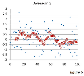
Here are some examples of how the averaging filter performs (figure 5)
One hundred random numbers were generated (blue dots) and a running averaging filter of size nine was applied. These are the red hollow squares. As can be observed, there is much lower variability in the squares than in the dots. Note that the solid squares would be the output of the block average and all the squares the output of the running average.
In general, this type of filter reduces noise by the square root of the number of samples.
Note the delay between the beginning of the filter and the appearance of the first output.
This is a plot of the same filter applied to the same data (figure 6), except the 26th datum was replaced by a noise spike (statistically referred to as an outlier). As mentioned before the averaging filter responds to outliers and as can be seen here samples 22 through 30 are affected by the outlier at location 26.
Lastly, is an example of the averaging filter’s response to a step-function (figure 7).


B. Median
The median is not calculated but rather, the measurements are sorted into ascending or descending order and, if an odd number of measurements are selected as the block size, the measurement in the middle is the median. If one selects an even number of measurements as the block size, the mean of the two most central ones is reported as the median.
The median filter is responsive to only one sample (ok, maybe 2 if it is an even block size) in the block being filtered. Since a high noise spike will never be in the median, the median filter is immune to individual high noises; the larger the block size, the less the effect of a high multisample noise spike.
Once a measurement is removed from the block and replaced with the newest one, that old measurement no longer has any effect on the returned result.
Here are some examples of how the median filter performs.
The same raw data as for the Averaging Filter (figure 8)
Similar improvement as the averaging filter but notice the somewhat strange stratification; the averaging filter uses all the data to produce its result, and the mean of a group of random numbers is rarely the same twice in a row. The median filter only uses one datum, the one in the sorted center, and sometimes that one datum will remain in the median location.
With the outlier (figure 9) notice that the median filter totally ignores the outlier.
Lastly, is an example of the median filter’s response to a step-function (figure 10); no slow constant ramp up and down.


C. Exponential
The exponential filter acts like a single-pole low pass filter (for the analog guys out there). It is calculated by (figure 11):
Where:
Result is the filtered value returned
t is the value at time t
t–1 is the value at the time just prior to t
Xt is the measurement at time t
The filter is initiated with Result t–1 and Xt both set to the first measurement.
Unlike the median and averaging filters, the exponential filter carries with it some remnant of every prior measurement; forever. Examining the equation, note that Result t–1 has 80% weight and the newest measurement (Xt) has only 20%. That having been stated, after a while the effects of old measurements carry smaller and smaller weight until they are practically no longer there.
Here are some examples of how the exponential filter performs.
The same raw data as for the prior filters (figure 12).
Similar improvement as the averaging filter notice that there is no delay from filter start to the appearance of the first result.
With the outlier (figure 13) there is some response to the outlier, but, unlike the averaging filter, this filter recovers smoothly rather than jumping up, staying up, and then jumping back down.
Lastly, is an example of the exponential filter’s response to a step-function; very analog like in nature (figure 14).


D. Attenuation
For Gaussian noise the averaging filter with length nine reduced the r.m.s. noise to 38%. The median filter reduced it to 52%, and the exponential to 37%. Note that longer filter lengths will allow the averaging and median filters to reduce the noise further. There is no equivalent adjustment for the exponential filter.
Which to choose? It depends entirely upon the application, but having multiple options available is a very nice thing.
If the lowest cost and most readily available device is adequate it may be foolish to spend more. On the other hand, if these characteristics matter in your circuit, measurements like these can save many problems.